6.2.5 Wind Speed Profiles

Dispersion models recommended for regulatory applications employ algorithms for extrapolating the input wind speed to the stack-top height of the source being modeled; the wind speed at stack-top is used for calculating transport and dilution. This section provides guidance for implementing these extrapolations using default parameters and recommends procedures for developing site specific parameters for use in place of the defaults.

For convenience, in non-complex terrain up to a height of about 200 m above ground level, it is assumed that the wind profile is reasonably well approximated as a power-law of the form:

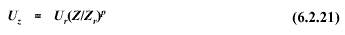
The power-law exponent for wind speed typically varies from about 0.1 on a sunny s afternoon to about 0.6 during a cloudless night. The larger the power-law exponent the larger the vertical gradient in the wind speed. Although the power-law is a useful engineering approximation of the average wind speed profile, actual profiles will deviate from this relationship.

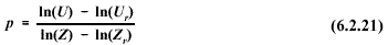
Site-specific values of the power-law exponent may be determined for sites with two levels of wind data by solving Equation (6.2.20) for p:

As discussed by Irwin [32], wind profile power-law exponents are a function of:

• stability,
• surface roughness
• the height range over which they are determined.

Hence, power-law exponents determined using two or more levels of wind measurements should be stratified by stability and surface roughness. Surface roughness may vary as a function of wind azimuth and season of the year (see Section 6.4.2). If such variations occur, this would require azimuth and season dependent determination of the wind profile power-law exponents. The power-law exponents are most applicable within the height range and season of the year used in their determination. Use of these wind profile power-law exponents for estimating the wind at levels above this height range or to other seasons should only be done with caution. The default values used in regulatory models are given in Table 6-2.

The following discussion presents a method for determining at what levels to specify the wind speed on a multi-level tower to best represent the wind speed profile in the vertical. The problem can be stated as, what is the percentage error resulting from using a linear interpolation over a height interval (between measurement levels), given a specified value for the power-law exponent. Although the focus is on wind speed, the results are equally applicable to profiles of other meteorological variables that can be approximated by power laws.

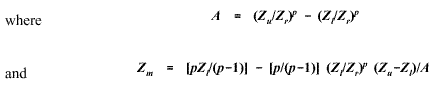
Let U_l represent the wind speed found by linear interpolation and U the "correct" wind speed. Then the fractional error is:

The fractional error will vary from zero at both the upper, Z_u , and lower, Z_l , bounds of the height interval, to a maximum at some intervening height, Z_m . If the wind profile follows a power law, the maximum fractional error and the height at which it occurs are: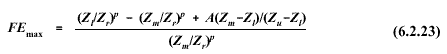

As an example, assume p equals 0.34 and the reference height, Z_r , is 10 m. Then for the following height intervals, the maximum percentage error and the height at which it occurs are:

As expected, the larger errors occur for the lower heights where the wind speed changes most rapidly with height. Thus, sensors should be spaced more closely together in the lower heights to best approximate the actual profile. Since the power-law is only an approximation of the actual profile, errors can occur that are larger than those estimated using (6.2.22). Even with this limitation, the methodology is useful for determining the optimum heights to place a limited number of wind sensors. The height Z_m represents the optimum height to place a third sensor given the location of the two surrounding sensors.

6. METEOROLOGICAL DATA PROCESSING
  6.1 Averaging and Sampling Strategies 
  6.2 Wind Direction and Wind Speed 
      6.2.1 Scalar Computations 
      6.2.2 Vector Computations 
      6.2.3 Treatment of Calms  
      6.2.4 Turbulence 
      6.2.5 Wind Speed Profiles  
  6.3 Temperature 
      6.3.1 Use in Plume-Rise Estimates  
      6.3.2 Vertical Temperature Gradient 
  6.4 Stability 
      6.4.1 Turner's method  
      6.4.2 Solar radiation/delta-T (SRDT) method 
      6.4.3  _E method 
      6.4.4 _Amethod 
      6.4.5 Accuracy of stability category estimates 
  6.5 Mixing Height 
      6.5.1 The Holzworth Method  
  6.6 Boundary Layer Parameters  
      6.6.1 The Profile Method 
      6.6.2 The Energy Budget Method  
      6.6.3 Surface Roughness Length 
      6.6.4 Guidance for Measurements in the Surface Layer 
  6.7 Use of Airport Data 
  6.8 Treatment of Missing Data  
      6.8.1 Substitution Procedures 
  6.9 Recommendations