6.6 Boundary Layer Parameters
This section provides recommendations for monitoring in support of air quality dispersion
models which incorporate boundary layer scaling techniques. The
applicability of these techniques is particularly sensitive to the
measurement heights for temperature and wind speed; the recommendations for
monitoring, given in Section 6.6.4, consequently, focus on the placement of
the temperature and wind speed sensors. A brief outline of boundary layer
theory, given in the following, provides necessary context for these
recommendations. The references for this section [48], [49], [50],
[51], [52], [53], [54], [55], [56],
[57], [58], [59] provide more detailed information on
boundary layer theory.
The
Atmospheric Boundary Layer (ABL) can be defined as the lower layer of the atmosphere,
where processes which contribute to the production or destruction of
turbulence are significant; it is comprised of two layers, a lower surface
layer, and a so-called mixed upper layer. The height of the ABL during
daytime roughly coincides with the height to which pollutants are mixed (the
mixing height, Section 6.5). During night-time stable conditions, the mixing
height (h) is an order of magnitude smaller than the maximum daytime value
over land; at night, h is typically below the top of the surface-based
radiation inversion [57].
The
turbulent structure of the ABL is determined by the amount of heat released
to the atmosphere from the earths surface (sensible heat flux) and by
interaction of the wind with the surface (momentum flux). This structure can
be described using three length scales: z (the height above the surface), h
(the mixing height ), and L (the MONIN - Obukhov length). The MONIN -
Obukhov length is
defined by:
- the surface fluxes of heat H =
pCp

- and momentum ,

and
reflects
the height at which contributions to the turbulent kinetic energy from
buoyancy and shear stress are comparable; the Obukhov length is defined as:
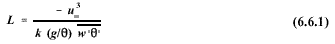
where
k is the von Karman constant,  is
the mean potential temperature within the surface layer, g/ is a buoyancy parameter, and u* is the friction velocity. The three
length scales define two independent non-dimensional parameters: a relative
height scale (z/h), and a stability index (h/L)[56].
is
the mean potential temperature within the surface layer, g/ is a buoyancy parameter, and u* is the friction velocity. The three
length scales define two independent non-dimensional parameters: a relative
height scale (z/h), and a stability index (h/L)[56].
Alternatives
to the measurement of the surface fluxes of heat and momentum for use in
(6.6.1) involve relating turbulence to the mean profiles of temperature and
wind speed.
The Richardson number, the ratio of thermal to mechanical
production (destruction) of turbulent kinetic energy, is directly related to
another non-dimensional stability parameter (z/L) and, thus, is a good
candidate for an alternative to 6.6.1. The gradient Richardson number (Rg)
can be approximated by:
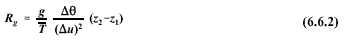
Large
negative Richardson numbers indicate unstable conditions while large
positive values indicate stable
conditions. Values close to zero are indicative of neutral conditions. Use
of (6.6.2) requires estimates of  u based on measurements of wind speed at
two levels in the surface layer; however, the level of accuracy required for
these measurements is problematic (u
is typically the same order of magnitude as the uncertainty in the wind
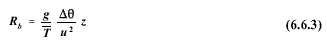
speed measurement). The bulk Richardson number (Rb ) which can be computed
with only one level of wind speed is a more practical alternative:
u based on measurements of wind speed at
two levels in the surface layer; however, the level of accuracy required for
these measurements is problematic (u
is typically the same order of magnitude as the uncertainty in the wind
speed measurement). The bulk Richardson number (Rb ) which can be computed
with only one level of wind speed is a more practical alternative:
6. METEOROLOGICAL DATA PROCESSING
6.1 Averaging and Sampling Strategies
6.2 Wind Direction and Wind Speed
6.2.1 Scalar Computations
6.2.2 Vector Computations
6.2.3 Treatment of Calms
6.2.4 Turbulence
6.2.5 Wind Speed Profiles
6.3 Temperature
6.3.1 Use in Plume-Rise Estimates
6.3.2 Vertical Temperature Gradient
6.4 Stability
6.4.1 Turner's method
6.4.2 Solar radiation/delta-T (SRDT) method
6.4.3
 E method
6.4.4 Amethod
6.4.5 Accuracy of stability category estimates
6.5 Mixing Height
6.5.1 The Holzworth Method
6.6 Boundary Layer Parameters
6.6.1 The Profile Method
6.6.2 The Energy Budget Method
6.6.3 Surface Roughness Length
6.6.4 Guidance for Measurements in the Surface Layer
6.7 Use of Airport Data
6.8 Treatment of Missing Data
6.8.1 Substitution Procedures
6.9 Recommendations